Dynamic Programming (Sutton & Barto)
- A collection of algorithms that can be used to compute optimal policies given a perfect model of the environment as an MDP.
- of limited utility in RL because of the assumption of a perfect model and their great computational expense, but still important theoretically.
- A common way of obtaining approximate solutions for tasks with continuous states and actions is to quantize the state and action spaces then apply finite-state DP methods.
- Key idea of DP: the use of value functions to organize and structure the search for good policies.
- DP algorithms are obtained by turning Bellman equations into update rules for improving approximations of the optimal value functions.
- Bootstrapping: All DP methods update estimates of the values of states based on estimates of the values of successor states. That is, they update estimates on the basis of other estimates.
4.1 Policy Evaluation
- Compute the state-value function $v_\pi$ for an arbitrary policy $\pi$.
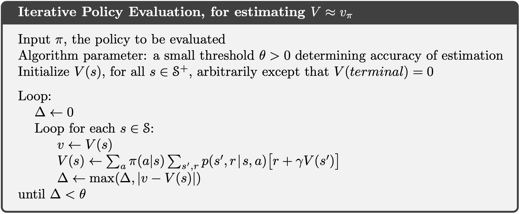
- The initial approximation $v_0$ is chosen arbitrarily, except that $v(terminal)=0$ $ \newcommand{\S}{\mathcal{S}} \newcommand{\A}{\mathcal{A}} \newcommand{\R}{\mathcal{R}} \newcommand{\E}{\mathrm{E}} \newcommand{\deq}{\dot{=}} \newcommand{\argmax}{\text{argmax }} \newcommand{\eps}{\varepsilon} $
- Use the Bellman equation for $v_\pi$ as an update rule
- The sequence \(\{v_k\}\) can be shown in general converge to $v_\pi$ as $k\rightarrow \infty$ under the same conditions that guarantee the existence of $v_\pi$.
- All the updates done in DP algorithms are called expected updates because they are based on an expectation over all possible next states rather than on a sample next state.
- Two types of implementation: two arrays vs. one array and update the values “in place”
- The in-place algorithm usually converges faster than the two-array version.
- Think of the updates as being done in a sweep through the state space.
- The iterative policy evaluation should be halted at some point: compute $\max_{s\in \S} \mid v_{k-1}(s)-v_k(s) \mid$ after each sweep and stops when it is sufficiently small.
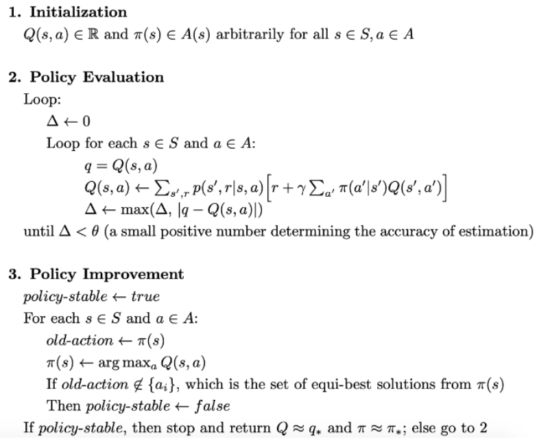
- Bellman equation as an update rule for $q$
4.2 Policy Improvement
- After finding the value function for a policy, we want to know whether or not we should change the policy to detereministically chose an action $a\neq \pi(s)$.
- Consider selecting action $a$ in state $s$ and thereafter following the existing policy $\pi$.
- If this is greater than $v_\pi(s)$, that is, if it is better to select $a$ once in $s$ and thereafter follow $\pi$ than it would be to follow $\pi$, then one would expect it to be better till to select $a$ every time $s$ is encountered. The new policy would in fact be a better one overall.
- Policy Improvement Theorem
If there are two determistic policies \(\pi\) and \(\pi^\prime\), and \(q_\pi(s, \pi^\prime(s)) \geq v_\pi(s) \text{ for all state } s \in \mathcal{S}\), then \(v_{\pi^\prime}(s) \geq v_\pi(s) \text{ for all } s \in \mathcal{S}\) ($\pi’$ is at least as good as $\pi$).
(Strict inequality) If \(q_\pi(s, \pi^\prime(s)) > v_\pi(s)\) for some state $s\in \S$, then \(v_{\pi^\prime}(s) > v_\pi(s)\). - Greedy policy $\pi’$
- The greedy policy $\pi’$ takes the action that looks best in the short term – after one step of lookahead – acoording to $v_\pi$. By construction, $\pi’$ meets the conditions of the policy improvement theorem, so it is at least as good as $\pi$.
- When $v_\pi=v_\pi’$, $v_\pi=v_\pi’=v_*$ and $\pi=\pi’$ is an optimal policy.
- Policy improvement gives us a strictly better policy except when the original policy is already optimal.
- The ideas can be extended to stochastic policies.
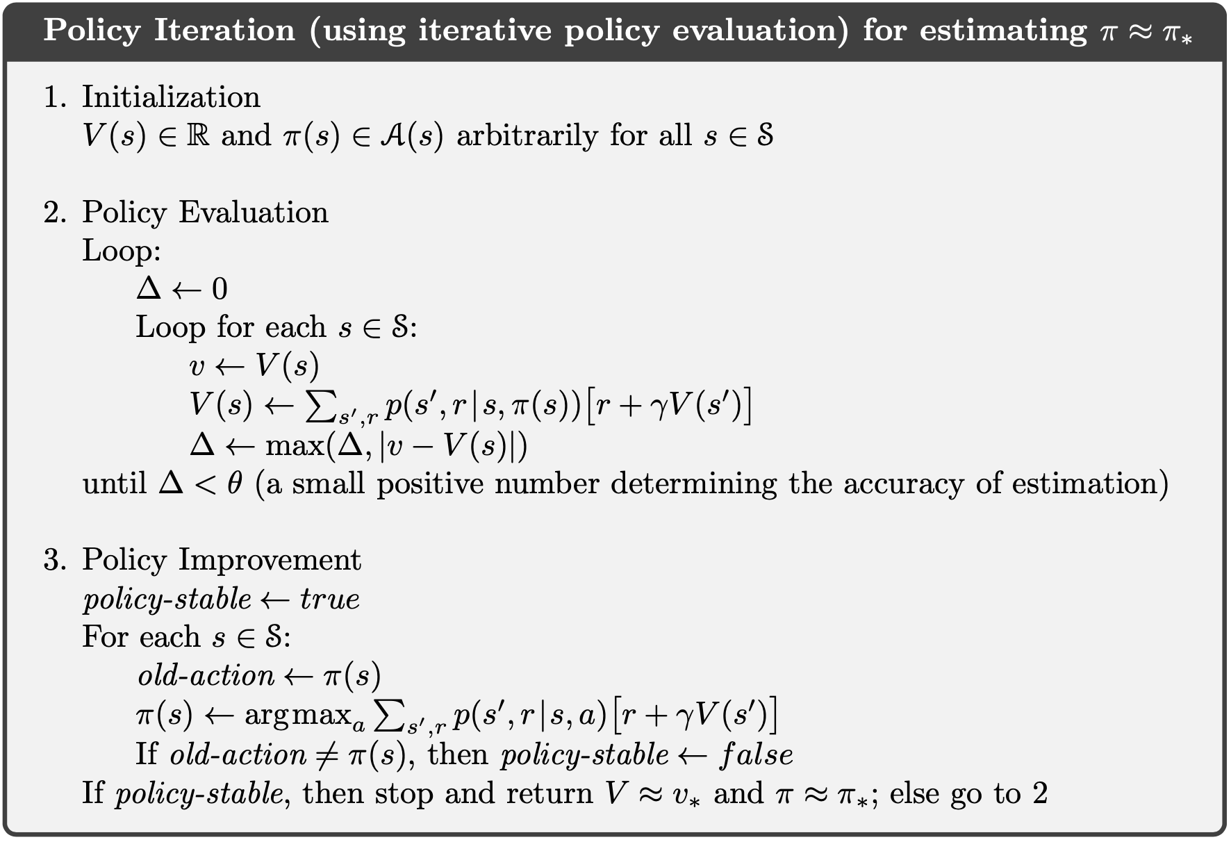
4.3 Policy Iteration
-
Once a policy, $\pi$, has been improved using $v_\pi$ to yield a better policy, $\pi’$, we can then compute $v_{\pi’}$ and improve it again to yield an even better $\pi’’$.

-
Because a finite MDP has only a finite number of policies, this process must converge to an optimal policy and optimal value function in a finite number of iterations.
-
Policy Iteration for action values
4.4 Value Iteration
- The policy evaluation step of policy iteration can be truncated in several ways without losing the convergence guarantees of policy iteration.
- In value iteration, policy evaluation is stopped after just one sweep.
- Can be written as a simple update operation that combines the policy improvement and truncated policy evaluation steps:
- obtained simply by turning the Bellman optimality equation into an update rule.
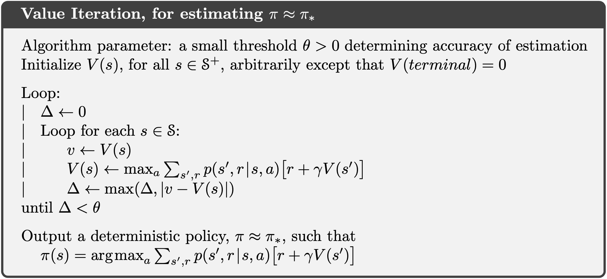
- effectively combines, in each sweeps, one sweep of policy evaluation and one sweep of policy improvement.
- Value iteration update for action values:
4.5 Asynchronous Dynamic Programming
- If the state set is very large, then even a single sweep can be prohibitively expensive.
- Asynchronous DP algorithms are in-place iterative DP algorithms that are not organized in terms of systematic sweeps of the state set.
4.6 Generalized Policy Iteration
- Policy iteration consists of two simultaneous, interacting processes, one making the value function consistent with the current policy (policy evaluation), and the other making the policy greedy with respect to the current value function (policy improvement)
- Generalized policy iteration: the general idea of letting policy-evaluation and policy-improvement processes interact.
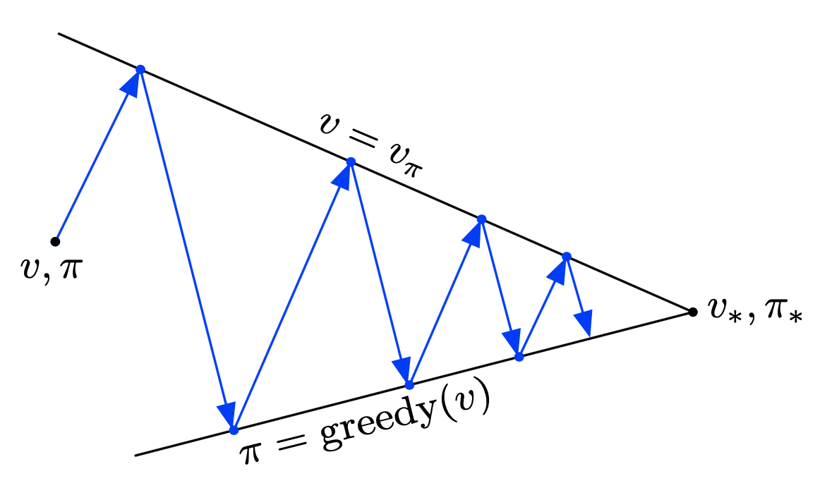
- The policy always being improved w.r.t the value function and the value function always being driven towards the value function for the policy.
- If both the evaluation process and the improvement process stabilize, that is, no longer produce changes, then the value function and policy must be optimal.
4.7 Efficiency of Dynamic Programming
- DP may not be practical for very large problems, but compared with other methods for solving MDPs, DP methods are actually quite efficient.
- On problems with large state spaces, asynchronous DP methods are often preferred.
References
- Richard S. Sutton and Andrew G. Barto. Reinforcement Learning: An Introduction; 2nd Edition. 2017.