Finite Markov Decision Processes (Sutton & Barto)
3.1 The Agent-Environment Interface
- MDPs: straightforward framing of the problem of learning from interaction to achieve a goal $ \newcommand{\S}{\mathcal{S}} \newcommand{\A}{\mathcal{A}} \newcommand{\R}{\mathcal{R}} \newcommand{\E}{\mathrm{E}} \newcommand{\deq}{\dot{=}} \newcommand{\argmax}{\text{argmax }} \newcommand{\eps}{\varepsilon} $
- Agent: learner/decision maker
- Environment: everything outside the agent
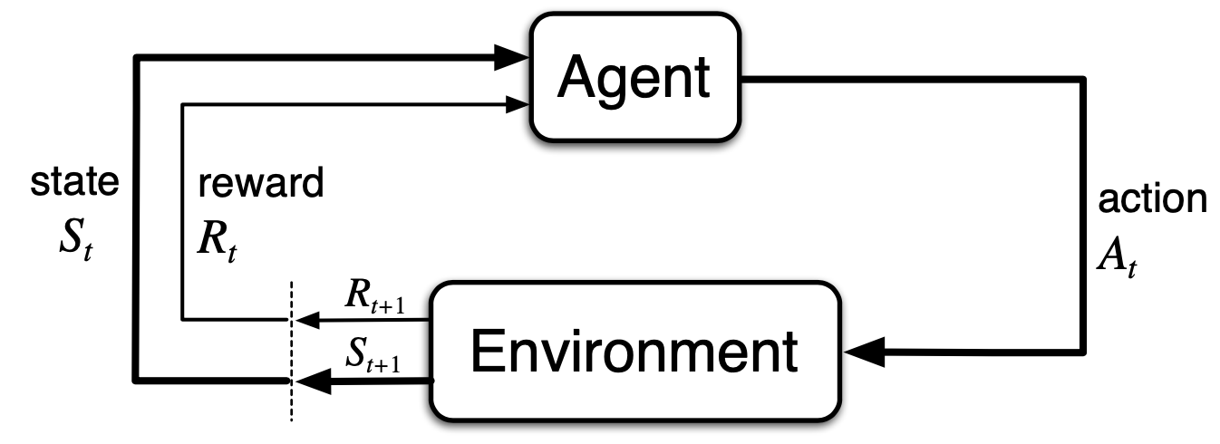
- Agent and environment interact at each time step $t$.
- At each time step t, the agent receives some representation of the environment’s state, $S_t\in \S$ and on that basis selects an action, $A_t\in \A(s)$
- One time step later, in part as a consequence of its action, the agent receives a numerical reward, $R_{t+1}\in \R$, and finds itself in a new state, $S_{t+1}$
- Sequence or trajectory: $S_0, A_0, R_1, S_2, A_2, R_2, …$
- In a finite MDP, all sets of states, actions, and rewards all have a finite number of elements
- Random variables $R_t, S_t$ have well defined discrete probability distribution dependent only on the preceding state $S_{t-1}$ and action $A_{t-1}$
- The function $p$ defines the dynamics of the MDP. A function of four arguments.
- By the axioms of probability,
- A state is said to have the Markov property if it includes information about all aspects of the past agent-environment interaction that make a difference for the future.
- State-transition probabilities
- Expected rewards for state-action pairs
- Expected rewards for state-action-next-state
- The general rule is that anything that cannot be changed arbitrary by the agent considered to be part of the environment
- The agent-evironment boundary represents the limit of the agent’s absolute control, not of its knowledge
- Actions represent the possible choices that can be made by the agent
- States represent the basis on which the choices are made
- Rewards define the agent’s goal
3.2 Goals and Rewards
- At each time step, the reward is a simple number $R_t \in \R$
- The agent’s goal is to maximize the total amount of reward it receives - the cumulative reward in the long run.
That all of what we mean by goals and purposes can be well thought of as the maximization of the expected value of the cumulative sum of a received scalar signal (called reward). (p.53)
- The agent always learns to maximize its reward. If we want it to do something for us, we must provide rewards to it in such a way that in maximizing them the agent will also achieve out goals.
- The reward signal is your way of communicating to the robot what you want it to achieve, not how you want it achieved.
3.3 Returns and Episodes
- Sequence of rewards received after time step $t$: $R_{t+1}, R_{t+2},…$
- Maximize the expected return $G_t=R_{t+1}+R_{t+2}+…+R_T$
- Episodes: subsequences of agent-environment interaction
- Terminal state: the state in which an episode ends
- Episodic tasks: tasks with episodes
- $\S$: the set of all nonterminal states
- $\S^+$: the set of all states plus the terminal state
- $T$: time of termination, a random variable varies from episode to episode
- Continuing tasks: Tasks in which the agent-environment interaction goes on continually without limit
- Discounting: the sum of the discounted rewards it receives over the future is maximized
- Expected discounted return
- $\gamma$ is called the discount rate
- If $\gamma<1$, the infinite sum has a finite value as long as the reward sequence \({R_k}\) is bounded.
- If $\gamma=0$, the agent is myopic in being concerned only with maximizing immediate rewards
- As $\gamma$ approaches 1, the return object takes future rewards into account more strongly; the agent becomes more farsighted
- Returns at successive time steps
- Define $G_T=0$
3.4 Unified Notation for Episodic and Continuing Tasks
- Consider episode termination to be the entering of a special absorbing state that transitions only to itself and that generates only rewards of zero.
- General notation of expected return
3.5 Policies and Value Functions
- Most RL algorithms involves estimating value functions - functions of states (or of state-action pairs) that estimate how good it is for the agent to be in a given state (or how good it is to perform a given action in a given state)
- The notion of “how good” is defined in terms of expected return
- Expected return depends on what actions the agent will take
- Value functions are defined with respect to particular ways of acting, called policies.
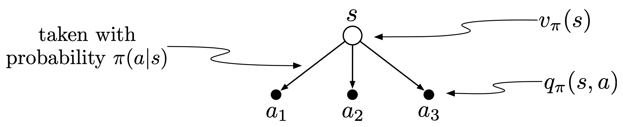
- Policy $\pi$: a mapping from states to probabilities of selecting each possible action
- If the agent is following policy $\pi$ at time $t$, $\pi(a\mid s)$ is the probability that $A_t=a$ if $S_t=s$.
- Reinforcement learning methods specify how the agent’s policy is changed as a result of its experience.
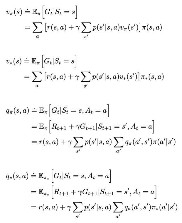
- State-value function for policy $\pi$ (Value function of a state $s$ under a policy $\pi$)
- Action-value function for policy $\pi$ (Value of taking action $a$ in state $s$ under a policy $\pi$)
- $v_\pi$ in terms of $q_\pi$
The value of a state depends on the values of the actions possible in that state and on how likely each action is to be taken under the current policy.
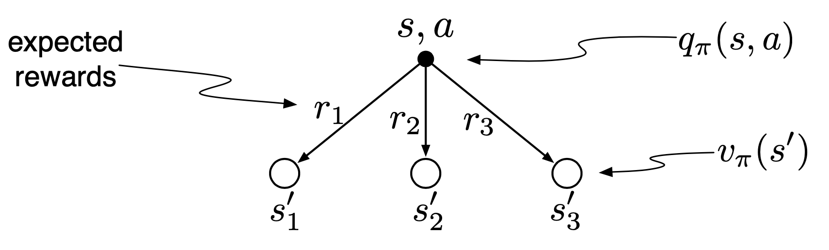
- $q_\pi$ in terms of $v_\pi$
The value of an action depends on the next reward, the values of the possible next states and on how likely it is to transition into each next state.
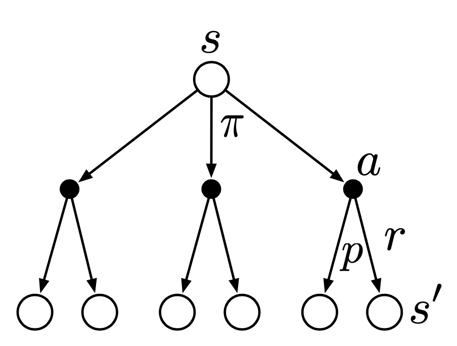
- Bellman equation for $v_\pi$: for any policy and state, the following consistency condition holds between the value of $s$ and the value of its possible successor states $s’$
- The Bellman equation states that the value of the start state must equal the (discounted) value of the expected next state, plus the reward expected along the way.
- Backup diagram for $v_\pi$
- Bellman equation for $q_\pi$
3.6 Optimal Policies and Optimal Value Functions
- A policy $\pi$ is defined to be better than or equal to a policy $\pi’$ if its expected return is greater than or equal to that of $\pi’$ for all states.
- Optimal policy $\pi_*$: There is always at least one policy that is better than or equal to all other policies.
- Optimal state-value function
- Optimal action-value function
- Because $v_*$ is the value function for a policy, it must satisfy the self-consistency condition given by the Bellman equation for state values.
- Because it is the optimal value function, it can be written without reference to any specific policy.
- Bellman optimality equation for $v_*$
- Bellman optimality equation for $q_*$
- For finite MDPs, the Bellman optimality equation for $v_*$ has a unique solution.
- If the dynamic function is given, it is actually a system of equations, one for each state.
- Once we have $v_*$, it is easy to determine an optimal policy: For each state s, there will be one or more actions at which the maximum is obtained in the Bellman optimality equation.
- Any policy that assigns nonzero probability only to these actions is an optimal policy.
- Any policy that is greedy with respect to the optimal evaluation function $v_*$ is an optimal policy.
- The optimal expected long-term return is turned into a quantity that is locally and immediately available for each state.
- With $q_* $, even easier: for any state $s$, simply choose an action that maximizes $q_* (s,a)$
- Hence, at the cost of representing a function of state-action pairs, instead of just of states, the optimal action-value function allows optimal actions to be selected without having to know anything about possible successor states and their values, that is, without having to know anything about the environment’s dynamics.
- Excplicitly solving the Bellman optimality equation is rarely useful as it assumes
- we accurately know the dynamics of the environment.
- we have enough computational resources to complete the computation of the solution.
- the Markov property.
- In RL we typically has to settle for approximate solutions.
- $v_* $ in terms of $q_* $
- $q_* $ in terms of $v_* $
- Other Bellman equations
References
- Richard S. Sutton and Andrew G. Barto. Reinforcement Learning: An Introduction; 2nd Edition. 2017.