Multi-armed Bandits (Sutton & Barto)
Difference between reinforcement learning and supervised learning
- RL: uses training information that evaluates the action taken
- SL: uses training information that instructs by giving correct actions
Two kinds of feedback
- Purely evaluative feedback: indicates how good the action taken was, but not whether it was the best or the worst action possible (depends entirely on action taken)
- Purely instructive feedback: indicates the correct action to take, independently of the action actually taken (independent of the action taken)
Nonassociative setting: setting that does not involve learning to act in more than one situation
2.1 The k-armed Bandit Problem
A nonassociative (does not involve learning to act in more than one situation), evaluative feed back problem.
Choose an action among k different options.
Receive a numerical reward chosen from a stationary probability distribution that depends on the action you selected.
Objective: maximize the expected total reward over some time period (e.g. 1000 action selections/time steps)
$ \newcommand{\E}{\mathrm{E}} \newcommand{\deq}{=} \newcommand{\argmax}{\text{argmax}} \newcommand{\eps}{\varepsilon} $ Action value
- The expected reward of a particular action
- $a$: a particular action
- $A_t$: action selected on time step $t$
- $R_t$: the corresponding reward
- $q_*(a)$: value of action $a$
- $q_*(a) \deq \E[R_t\mid A_t=a]$
Estimated action value
- $Q_t(a)$: estimated action value
- Want $Q_t(a)$ to be close to $q_*(a)$
- Greedy action: an action whose estimated value is greatest
- Exploitation: select a greedy action
- Exploration: select a nongreedy action (enables you to improve your estimate of the nongreedy action’s value)
Exploitation vs Exploration
- Exploitation maximizes the expected reward on the one step, but exploration may produce the greater total reward in the long run.
- Reward is lower in the short run, during exploration, but higher in the long run because after you have discovered the better actions, you can exploit them many times. Exploration-exploitation conflict: not possible both to explore and to exploit with any single action selection
- Balancing exploration and exploitation: deciding when to explore/exploit
2.2 Action-vlue Methods
- Methods for estimating the valuyes of actions and for using the estimates to make action selection decisions
- Estimating the expected reward of an action by averaging the rewards actually received
- As the denominator goes to infinity, by the law of large numbers, $Q_t(a)$ converges to $q_*(a)$.
- The sample-average method for estimating action values
Greedy action selection method
- Always select one of the actions with the highest estimated value
$\eps$-greedy Method
- Behave greedily most of the time, but with small probability $\eps$, selecting randomly from among all the actions with equal probability.
- Advantage: As the number of steps increases, every action will be sampled an infinite number of times, $Q_t(a)$ converges to $q_*(a)$.
2.3 The 10-armed Testbed
- 10 actions: $a=1,…,10$
- $q_*(a)$: Normal(0,1)
- Learning method: greedy/$\eps$- greedy(0.01)/$\eps$-greedy(0.1)
- $R_t$: Normal($q_*(A_t)$,1)
- Calculate $Q_t(a)$ using sample-average method
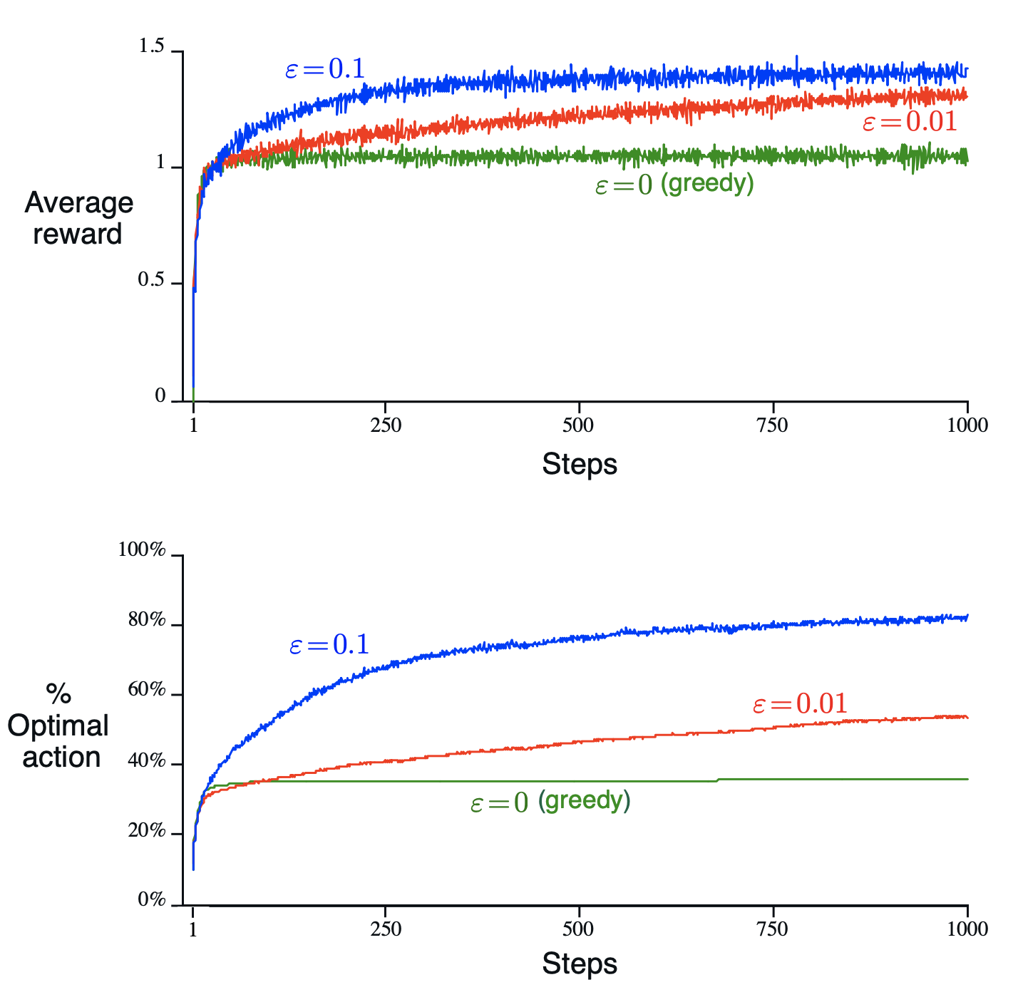
- The greedy method found the optimal action in only approximately one-third of the tasks.
- The $\eps$=0.1 method expored more, and usually found the optimal action earlier, but never selected that action more than 91% of the time
- The $\eps$=0.01 method improved more slowly but eventually would perform better than the epsilon=0.1 method.
- Possible to reduce epsilon over time to try to get the best of both high and low values.
- Larger variance: takes more exploration to find optimal action
- Zero variance: greedy method might perform best
- If the bandit task is nonstationary (action values changed over time) but deterministic (variance=0), exploration is needed to make sure one of the nongreedy actions has not changed to become better than the greedy one.
- Nonstationary is the case most commonly encountered in reinforcement learning: the learner faces a set of banditlike decision tasks each of which changes over time as learning proceeds and the agent’s decision-making policy changes.
2.4 Incremental Implementation
- How to compute estimated action value with simple-average method efficiently with constant memory and constant per-time-step computation?
- $R_i$ = reward received after the $i$-th selection of an action
- $Q_n$ = estimate of its action value after it has been selected $n-1$ times = $\frac{R_1+…+R_{n-1}}{n-1}$
- If we maintain a record of all the rewards, memory and computational requirements will grow over time.
- Instead, we can use an incremental formula for updating averages
NewEstimate ← OldEstimate + StepSize [Target - OldEstimate]- The expression
Target - OldEstimateis an error in the estimate
A simple bandit algorithm
Initialize, for $a=1$ to $k$:
$\quad Q(a) \leftarrow 0$
$\quad N(a) \leftarrow 0$
Loop forever:
\(\quad A \leftarrow \begin{cases} \argmax_a Q(a) && \text{with probability } 1 - \eps\\ \text{a random action} && \text{with probability } \eps \end{cases}\)
$\quad R \leftarrow bandit(A)$
$\quad N(A) \leftarrow N(A)+1$
$\quad Q(A) \leftarrow Q(A) + \frac{1}{N(A)}[R-Q(A)]$
2.5 Tracking a Nonstationary Problem
- We often encounter reinforcement learning problems that are effectively nonstationary.
- It makes sense to give more weight to recent reward than to long-past rewards.
- One of the most popular ways of doing this is to use a constant step-size parameter.
- We call this a weighted average of past rewards and the initial estimate $Q_1$ because the sum of the weights $(1-\alpha)^n+\sum_{i=1}^n \alpha(1-\alpha)^{n-i}=1$
- This is sometimes called an exponential recency-weighted average
- Conditions for convergence with probability 1:
- Generalized exponential recency-weighted average (if step-size parameters $\alpha_n$ are not constant)
2.6 Optimistic Initial Values
- Initial bias: disappears once all acitons have been selected at least once for sample-average methods; permanent though decreasing over time for constat step-size methods
- Setting the initial estimated action values optimistically to encourage exploration
- The system does a fair amount of exploration even if greedy actions are selected all the time
- Not well suited to nonstationary problems because its drive for exploration is inherently temporary.
2.7 Upper-Confidence-Bound Action Selection (UCB)
- Select actions according to $A_t = \argmax_a \left[Q_t(a) + c\sqrt{\frac{\ln t}{N_t(a)}} \right]$
- It would be better to select among the non-greedy actions according to their potential for actually being optimal, taking in account both how close their estimates are to being maximal and the uncertainties in those estimates.
- All actions will eventually be selected, but actions with lower value estimates, or that have already been selected frequently, will be selected with decreasing frequency over time.
2.8 Gradient Bandit Algorithms
2.9 Associative Search (Contextual Bandits)
- Nonassociative tasks: tasks in which there is no need to associate different actions with different situations.
- In general reinforcement learning task there is more than one situation, and the goal is to learn a policy: a mapping from situations to the actions that are best in those situations.
- Suppose there are several different k-armed bandit tasks, and that on each step you confront one of these chosen at random.
- Associative search task: involves both trial-and-error learning to search for the best actions, and association of these actions with the situations in which they are best. (Contextual bandits)
- An intermediate between the k-armed bandit problem and the full reinforcement learning problem: like the full reinforcement learning problem in that they involve learning a policy, but like the k-armed bandit problem in that each action affects only the immediate reward.
References
- Richard S. Sutton and Andrew G. Barto. Reinforcement Learning: An Introduction; 2nd Edition. 2017.