Prediction and Control with Function Approximation (Coursera)
Parametrizing the Value Function
\[\newcommand{\bm}[1]{\textbf{#1}} \newcommand{\w}{\bm{w}} \newcommand{\vhat}{\hat{v}} \vhat(s, \w) \approx v_\pi(s)\]Linear Value Function Approximation
\[\newcommand{\x}{\bm{x}} \begin{align*}\vhat(s,\w) \doteq & \sum w_i x_i(s)\\ = & <\w, \x(s)>\end{align*}\]Tabular representation is a special case of linear function approximation
\[\vhat(s, \w) = <\w, \x(s_i)> = w_i\]where $\x(s_i)$ is a one-hot vector and $w_i$ is the state value in the table.
The Value Error Objective
\[\newcommand{\VE}{\overline{VE}}\VE=\sum_s\mu(s)[v_\pi(s)-\vhat(s,\w)]^2\]$\mu(s)$ is the fraction of time state $s$ is visited under the policy.
Gradiant Descent
\[\w_{t+1}\doteq \w_t -\alpha \nabla J(w_t)\]- The global minimum does not necessarily correspond to the true value function.
- Limited by the choice of function parameterization, depends on the choice of objective.
Gradient of a Linear Value Function
\[\vhat(s,\w)\doteq \sum w_i x_i(s)\] \[\newcommand{\pp}[2]{\frac{\partial{#1}}{\partial{#2}}} \pp{\vhat(s,\w)}{w_i}=x_i(s)\] \[\nabla\vhat (s,\w)=\x(s)\]Gradient of $\VE$
\[\begin{align*} \nabla \VE &= \nabla \sum_{s\in S} \mu(s)[v_\pi(s)-\vhat(s,\w)]^2\\ &= \sum_{s\in S} \mu(s)\nabla [v_\pi(s)-\vhat(s,\w)]^2\\ &= -\sum_{s\in S} \mu(s) 2[v_\pi(s)-\vhat(s,\w)] \nabla \vhat(s,\w)\\ \end{align*}\]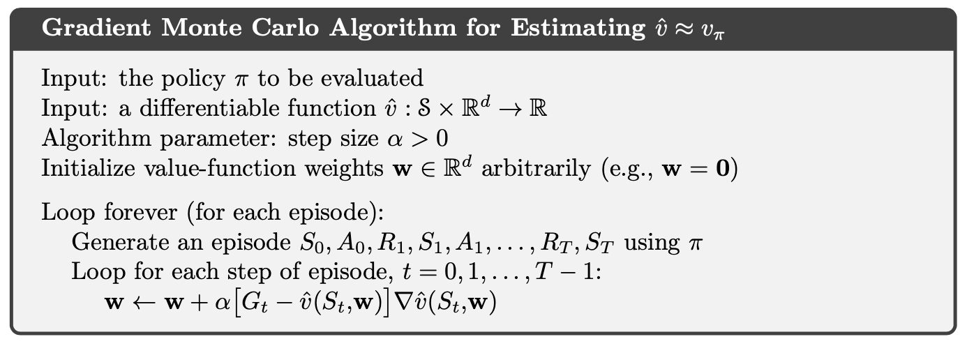
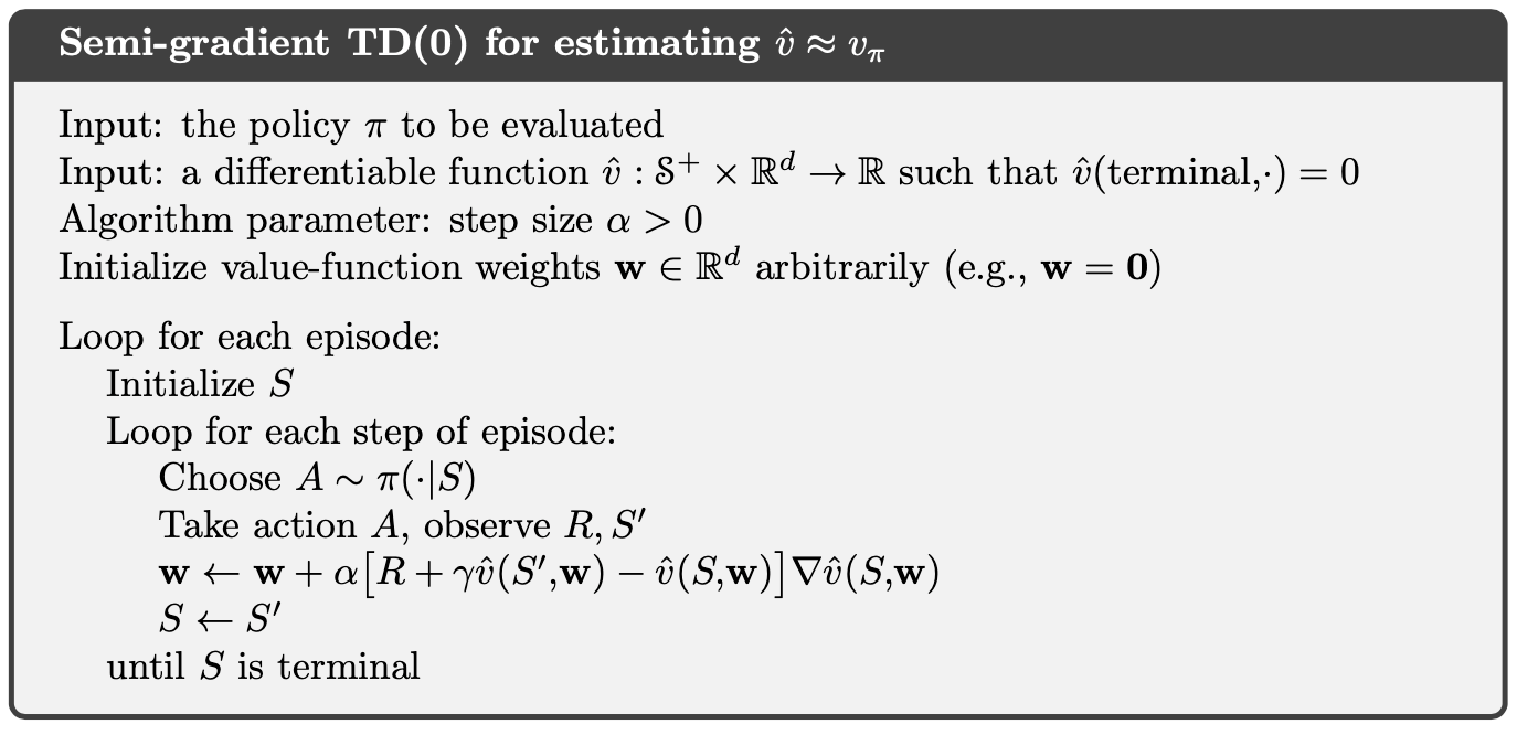
The TD Update for Function Approximation
\[\w \leftarrow \w + \alpha [\underbrace{R_{t+1}+\gamma \vhat(S_{t+1}, \w)}_{U_t} - \vhat(S_t,\w)] \nabla \vhat(S_t, \w)\]- The TD target $U_t$ is biased but often has lower variance than the sample of the return.
- TD does not have to wait until the end of an episode to make updates.
- Will not necessarily converge to a local minimum of $\VE$.
- Often learn faster than Monte Carlo because TD can learn during the episode and has lower variance updates.
Episodic Sarsa with Function Approximation
\[\newcommand{\qhat}{\hat{q}} \w \leftarrow \w +\alpha[R+\gamma \qhat(S',A',\w) - \qhat(S,A,\w)] \nabla \qhat(S,A,\w)\]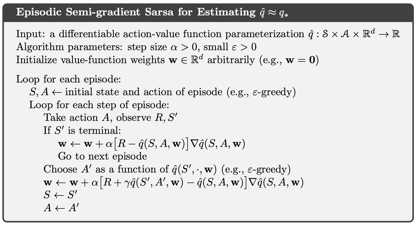
Sarsa/Q-learning with Function Approximation
Sarsa:
\[Q(S_t, A_t)\leftarrow Q(S_t, A_t) +\alpha(R_{t+1}+\gamma Q(S_{t+1}, A_{t+1})-Q(S_t, A_t))\]Expected Sarsa:
\[Q(S_t, A_t)\leftarrow Q(S_t, A_t) +\alpha(R_{t+1}+ \gamma \sum_{a'} \pi(a' | S_{t+1})Q(S_{t+1}, a')-Q(S_t, A_t))\]Sarsa with function approximation:
\[\w \leftarrow \w +\alpha(R_{t+1}+\gamma \qhat(S_{t+1}, A_{t+1}, \w)-\qhat(S_t, A_t, \w)) \nabla \qhat(S_t, A_t, \w)\]Expected Sarsa with function approximation:
\[\w \leftarrow \w +\alpha(R_{t+1}+\gamma \sum_{a'} \pi(a' | S_{t+1}) \qhat(S_{t+1}, a', \w)-\qhat(S_t, A_t, \w)) \nabla \qhat(S_t, A_t, \w)\]Q-learning with function approximation:
\[\w \leftarrow \w + \alpha (R_{t+1}+\gamma \max_a' \qhat (S_{t+1}, a', \w) - \qhat (S_t, A_t, \w)) \nabla \qhat(S_t, A_t, \w)\]Average Reward
\[\newcommand{\E}{\mathbb{E}} \begin{align*} r(\pi)\doteq & \lim_{h\rightarrow \infty} \frac{1}{h} \sum_{t=1}^{h} \E[R_t|S_0,A_{0:t-1} \sim \pi]\\ = & \sum_s \mu_\pi(s) \sum_a \pi(a|s) \sum_{s',r} p(s',r|s,a) r \end{align*}\]Value Function for Average Reward
\[\begin{align*}q_\pi(s,a)&=\E_\pi[G_t|S_t=s,A_t=a]\\ &=\E_\pi[R_{t+1}-r(\pi)+R_{t+2}-r(\pi)+ \dots|S_t=s,A_t=a]\\ &=\sum_{s', r} p(s',r|s,a)(r-r(\pi)+v_\pi(s'))\\ &=\sum_{s', r} p(s',r|s,a)(r-r(\pi)+\sum_{a'}\pi(a'|s')q_\pi(s',a'))\end{align*}\]The Softmax Policy Parameterization
\[\newcommand{\t}{\boldsymbol{\theta}} \newcommand{\A}{\mathcal{A}} \pi(a|s, \t) \doteq \frac{e^{h(s,a,\t)}}{\sum_{b\in \A} e^{h(s,b,\t)}}\]- $h(s,a,\t)$ is the action preference.
- Exponentiation to ensure each action has a positive probability.
- A softmax policy over action preferences can behave very differently than the epsilon-greedy policy derived from action values.
Advantages of Policy Parameterization
- Agents can autonomously decrease exploration over time.
- Agents can avoid failure to deterministic policies with limited function approximation
- Policy is sometimes less copmlicated than value function.
The Average Reward Objective
Find $\t$ for which
\[r(\pi)=\sum_s \mu(s) \sum_a \pi(a|s,\t) \sum_{s',r} p(s',r|s,a)r\]is maximized.
The Policy Gradient
\[\nabla r(\pi) = \nabla \sum_s \mu(s)\sum_a \pi(a|s,\t) \sum_{s', r} p(s',r|s,a)r\]The Policy Gradient Theorem
\[\nabla r(\pi) = \sum_s \mu(s) \sum_a \nabla \pi(a|s,\t) q_\pi(s,a)\]Stochastic Gradient Ascent for Policy Parameters
\[\begin{align*} \nabla r(\pi) &= \sum_s \mu(s) \sum_a \nabla \pi(a|s,\t) q_\pi(s,a)\\ &= \E_\pi [\sum_a \nabla \pi(a|S, \t)q_\pi(S,a)]\\ &= \E_\pi [\sum_a \pi(a|S,\t)\frac{1}{\pi(a|S,\t)} \nabla \pi(a|S, \t)q_\pi(S,a)]\\ &= \E_\pi [\E_\pi [\frac{\nabla \pi(A|S, \t)}{\pi(A|S, \t)}q_\pi(S,A)]]\\ &= \E_\pi [\frac{\nabla \pi(A|S, \t)}{\pi(A|S, \t)}q_\pi(S,A)]\\ &= \E_\pi [\nabla \ln \pi(A|S, \t) q_\pi(S,A)] & \because \nabla \ln(f(x))=\frac{\nabla f(x)}{f(x)} \end{align*}\]Therefore, the update rule for stochastic gradient ascent is
\[\t_{t+1} \leftarrow \t_t+\alpha \nabla \ln \pi(A_t|S_t,\t_t) q_\pi(S_t, A_t)\]Actor-Critic Algorithm
Using $\newcommand{\Rbar}{\overline{R}} R_{t+1}-\Rbar+\vhat(S_{t+1},\w)$ to approximate the action value $q_\pi(S_t, A_t)$,
\[\t_{t+1} = \t_t+\alpha \nabla \ln \pi(A_t|S_t,\t_t) [R_{t+1}-\Rbar+\vhat(S_{t+1},\w)]\]Adding a baseline tends to reduces the update variance
\[\t_{t+1} = \t_t+\alpha \nabla \ln \pi(A_t|S_t,\t_t) [\underbrace{R_{t+1}-\Rbar+\vhat(S_{t+1},\w)\color{red}{-\vhat(S_t, \w)}}_{\delta_t}]\]The rule for updating the state value function is (same as before)
\[\w \leftarrow \w + \alpha^\w \delta \nabla \vhat(S, \w)\]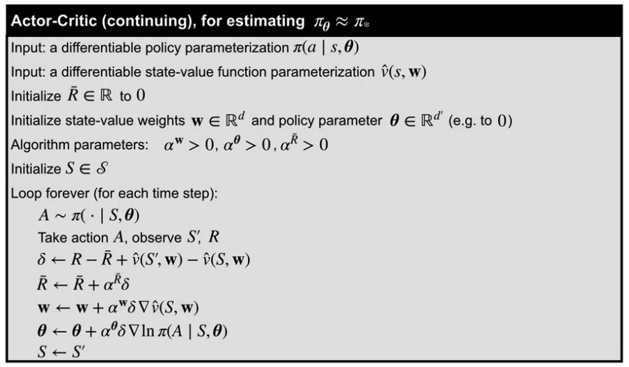
Using a softmax policy
\[\pi(a|s,\w)\doteq \frac{e^{h(s,a,\w)}}{\sum_{b\in \A}e^{h(s,b,\w)}}\]and linear function approximators
\[\vhat(s,\w)\doteq \w^T\x(s)\] \[h(s,a,\w)\doteq \t^T \x_h(s,a)\]the gradients are
\[\nabla \vhat(s,\w) = \x(s)\] \[\begin{equation}\label{eq:pg} \nabla \ln \pi(a|s,\t) = \x_h(s,a) - \sum_b \pi(b|s,\t) \x_h(s,b) \end{equation}\]Derivation for $(\ref{eq:pg})$:
\[\begin{align*} \nabla \ln \pi(a|s,\t) & = \nabla \ln \frac{e^{h(s,a,\t)}}{\sum_b e^{h(s,b,\t)}}\\ & = \nabla h(s,a,\t) -\nabla \ln \sum_b e^{h(s,b,\t)}\\ & = \x_h(s,a) - \frac{1}{\sum_{b'} e^{h(s,b',\t)}} \nabla \sum_b e^{h(s,b,\t)}\\ & = \x_h(s,a) - \frac{1}{\sum_{b'} e^{h(s,b',\t)}} \nabla \sum_b e^{\t^T \x_h(s,b)}\\ & = \x_h(s,a) - \frac{1}{\sum_{b'} e^{h(s,b',\t)}} \sum_b e^{\t^T \x_h(s,b)}\x_h(s,b)\\ & = \x_h(s,a) - \sum_b \frac{e^{\t^T \x_h(s,b)}}{\sum_{b'} e^{h(s,b',\t)}} \x_h(s,b)\\ & = \x_h(s,a) - \sum_b \pi(b|s,\t) \x_h(s,b)\\ \end{align*}\]Gaussian Policies for Continuous Actions
\[\newcommand{\exp}{\text{exp}} \pi(a|s,\t) \doteq \frac{1}{\sigma(s,\t)\sqrt{2\pi}}\exp(-\frac{(a-\mu(s,\t))^2}{2\sigma(s,\t)^2})\] \[\mu(s,\t)\doteq \t^T_\mu \x(s)\] \[\sigma(s,\t) \doteq \exp(\t^T_\sigma \x(s) )\]The gradients are
\[\begin{equation}\label{eq:mu} \nabla \ln \pi(a|s, \t_\mu) = \frac{1}{\sigma(s,\t)^2}(a-\mu(s,\t))\x(s)\end{equation}\] \[\begin{equation}\label{eq:sigma} \nabla \ln \pi(a|s, \t_\sigma) = \left (\frac{(a-\mu(s,\t))^2}{\sigma(s, \t)^2}-1 \right )\x(s)\end{equation}\]Derivation for $(\ref{eq:mu})$:
\[\begin{align*} \nabla \ln \pi(a|s, \t_\mu) &= \nabla_{\t_\mu} \ln \frac{1}{\sigma \sqrt{2\pi}} e^{-(a-\mu)^2/2\sigma^2} \\ &= \nabla_{\t_\mu}\left[ \ln \frac{1}{\sigma \sqrt{2\pi}} + \ln e^{-(a-\mu)^2/2\sigma^2} \right]\\ &= \nabla_{\t_\mu}\ln e^{-(a-\mu)^2/2\sigma^2}\\ &= \nabla_{\t_\mu} -(a-\mu)^2/2\sigma^2\\ &= -\frac{1}{2\sigma^2} \nabla_{\t_\mu} (a-\mu)^2\\ &= \frac{1}{2\sigma^2} 2(a-\mu) \nabla_{\t_\mu} \mu\\ &= \frac{a-\mu}{\sigma^2} \x \end{align*}\]Derivation for $(\ref{eq:sigma})$:
\[\begin{align*} \newcommand{\gradsig}{\nabla_{\t_\sigma}} \nabla \ln \pi(a|s, \t_\sigma) &= \gradsig \ln \frac{1}{\sigma \sqrt{2\pi}} e^{-(a-\mu)^2/2\sigma^2} \\ &= \gradsig \left[ \ln \frac{1}{\sigma \sqrt{2\pi}} + \ln e^{-(a-\mu)^2/2\sigma^2} \right]\\ &= -\gradsig\ln(\sigma \sqrt{2\pi}) + \gradsig \frac{-(a-\mu)^2}{2\sigma^2} \\ &= -(\gradsig\ln(\sigma) + \gradsig \ln(\sqrt{2\pi})) + \gradsig \frac{-(a-\mu)^2}{2\sigma^2} \\ &= -\frac{\gradsig \sigma}{\sigma}-\frac{(a-\mu)^2}{2}\gradsig \sigma^{-2}\\ &= -\frac{\sigma \x}{\sigma}-\frac{(a-\mu)^2}{2}(-2) \sigma^{-3} \gradsig \sigma\\ &= -\x+(a-\mu)^2 \sigma^{-3}\sigma \x\\ &= \left[\frac{(a-\mu)^2}{\sigma^2}-1\right]\x\\ \end{align*}\]