- require only experience - sample sequences of states, actions, rewards from actual or simulated interaction with an environment
- Methods based on averaging sample returns from complete episodes.
- Only on the completion of an episode are value estimates and policies changed.
- DP methods compute value functions from knowledge of MDP. MC methods learn value functions from sample returns with the MDP.
- No MDP knowledge (Without model). Only simple experience is available.
- Only works for episodic environments
5.1 Monte Carlo Prediction
- To learn the value function for a given policy.$
\newcommand{\S}{\mathcal{S}}
\newcommand{\A}{\mathcal{A}}
\newcommand{\R}{\mathcal{R}}
\newcommand{\E}{\mathrm{E}}
\newcommand{\deq}{\dot{=}}
\newcommand{\argmax}[1]{\text{argmax}_{#1} \text{ }}
\newcommand{\eps}{\varepsilon}
\newcommand{\N}{\text{Normal}}
\newcommand{\p}{\rho}
\newcommand{\T}{\mathbb{T}}
$
- The value of a state is the expected return starting from that state.
- An obvious way to estimate it from experience is to average the returns observed after visits to that state.
- Given $a$ set of episodes obtained by following $\pi$ and passing through $s$. Each occurrence of state $s$ in an episode is called a visit to $s$.
- In first-vist MC policy evaluation, we estimates $v_\pi(s)$ as the average of the returns following first visits to $s$.
- In every-visit MC policy evaluation, we averages the returns following all visits to $s$.
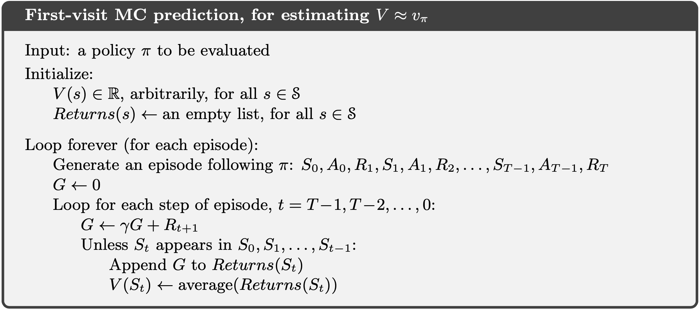
- Each return is an independent, identically distributed estimate of $v_\pi(s)$ with finite variance. By the law of large numbers the sequence of averages of these estimates converges to their expected value.
- The estimates for each state are independent - does not build upon the estimate of any other state, as is the case in DP.
- MC methods are model-free and do not bootstrap.
- The computational expense of estimating the value of a single state is independent of the number of states.
- Can generate many sample episodes starting from the states of interest, averaging returns from only these states, ignoring all others.
5.2 Monte Carlo Estimation of Action Values
- If a model is not available, then it is particularly useful to estimate aciton values rather than state values.
- State values alone are not sufficient to determine a policy without a model.
- Policy evaluation for action values: the expected return when starting in state $s$, taking action $a$, and thereafter folloing poliocy $\pi$
- The Monte Carlo methods for this are essentially the same as just presented for state values, except now we talk about visits to state-action pair rather than to a state. A state-action pair $s,a$ is said to be visited in an episode if ever the state $s$ is visited and action $a$ is taken in it.
- If $\pi$ is a determinitic policy, then in following $\pi$ one will observe returns only for one of the actions from each state. To compare alternatives we need to estimate the value of all the acitons form each state, not just the one we currently favor.
- For policy evaluation to work for action values, we must assure continual exploration.
- One way to do this is by specifying that the episodes start in a state-action pair, and that every pair has a nonzero probability of being selected as the start. We call this the assiumption of exploring starts.
- Another approach to assuring that all state-action pairs are encountered is to consider only policies that are stochastic with a nonzero probability of selecting all actions in each state.
5.3 Monte Carlo Control
- Perform alternating complete steps of policy evaluation and policy improvement, beginning with an arbitrary policy $\pi_0$ and ending with the optimal policy and optimal ation-value function.

- For any action-value function $q$, the corresponding greedy policy is the one that, for each $s \in \S$, deterministically chooses an action with maximal action-value:
\[\pi(s)=\argmax{a} q(s,a)\]
- For Monte Carlo Policy iteration it is natural to alternate between evaluation and improvement on an episode-by-episode basis.
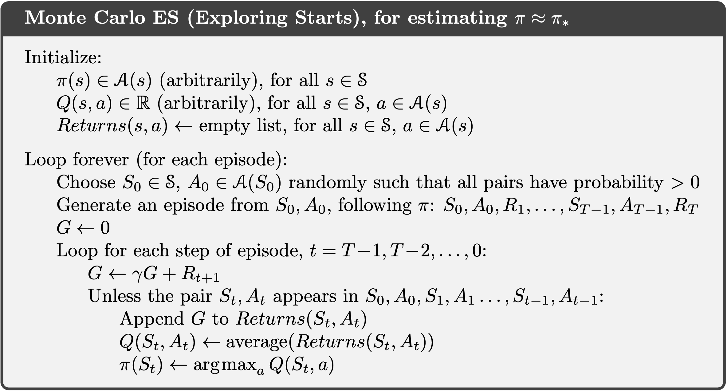
- To update the mean incrementally,
\[Q_{n+1}=Q_n+\frac{1}{n}(R_n-Q_n)\]
5.4 Monte Carlo without Exploring Starts
- How to avoid exploring starts but still ensure that all ations are selected infinitely often?
- Two approaches: On-policy methods attempt to evaulate or improve the policy that is used to make decisions, whereas off-policy methods evaluate or improve a policy different from that used to generate the data.
- In on-policy control methods the policy is generally soft, meaning that $\pi(a\mid s)>0$ for all $s \in \S$ and all $a \in \A(s)$, but gradually shifted closer and closer to a deterministic optimal policy.
- $\eps$-greedy policies: all nongreedy actions are given the minimal probability of selection, $\eps/\mid A(s)\mid$, and then remaining bulk of the probability, $1-\eps + \eps/\mid A(s)\mid$, is given to the greedy action.
- $\eps$-soft policy: policies for which $\pi(a\mid s)>\eps/\mid A(s)\mid$ for all states and actions, for some $\eps>0$.
- For any $\eps$-soft policy, any $\eps$-greedy policy with respect to $q_\pi$ is guaranteed to be better than or equal to $\pi$.
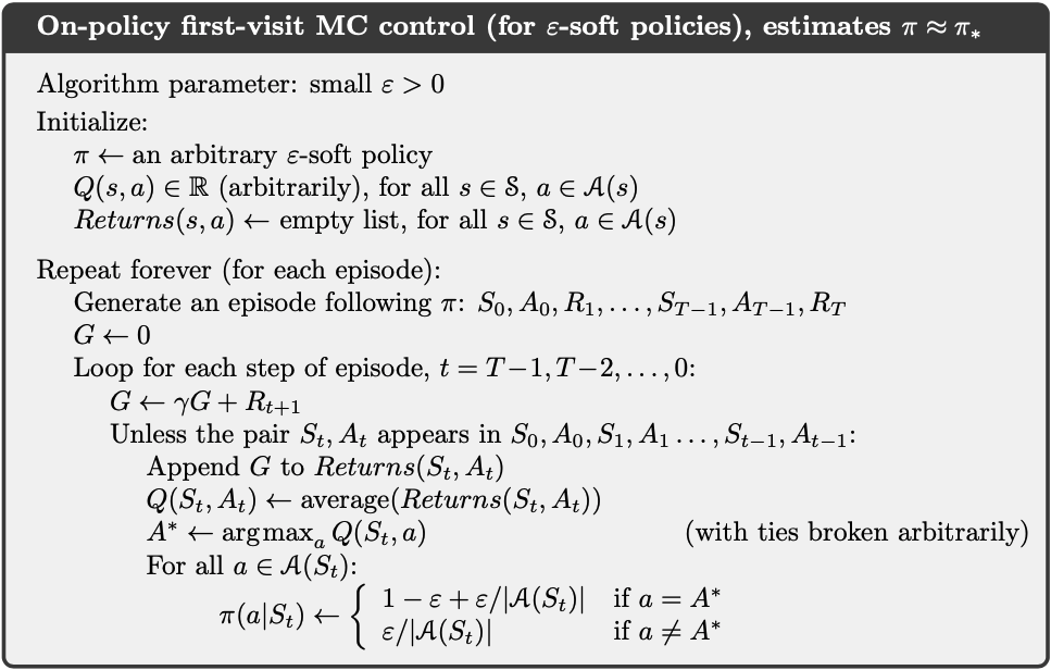
- That any $\eps$-greedy policy w.r.t. $q_\pi$ is an improvement over any $\eps$-soft polict $\pi$ is assured by the policy improvement theorem. $\pi’ \geq \pi$, where $\pi’$ is an $\eps$-greedy policy w.r.t. $q_\pi$.
- Equality can hold only when both $\pi’$ and $\pi$ are optimal among the $\eps$-soft policies.
- This analysis is independent of how the action-value functions are determined at each stage, but it does assume that they are computed correctly.
- Now we only achieve the best policy among the epsilon-soft policies, but on the other hand, we have elimited the assumption of exploring starts.
5.5 Off-policy Prediction via Importance Sampling
- All learning control methods face a dilemma: They seek to learn action values conditional on subsequent optimal behavior, but they need to behave non-optimally in order to explore all actions (to find optimal actions).
- On-policy approach: learn action values for a near-optimal policy that still explores.
- Off-policy approach: use two policies, one that is learned about and that becomes the optimal policy, and one that is more exploratory and is used to generate behavior.
- Target policy: the policy being learned about
- Behavior policy: the policy used to generate behavior
- Learning is from data “off” the policy
- Off-policy methods are more powerful and general.
- Off-policy methods include on-policy methods as the specifal case in which the target and behavior policies are the same.
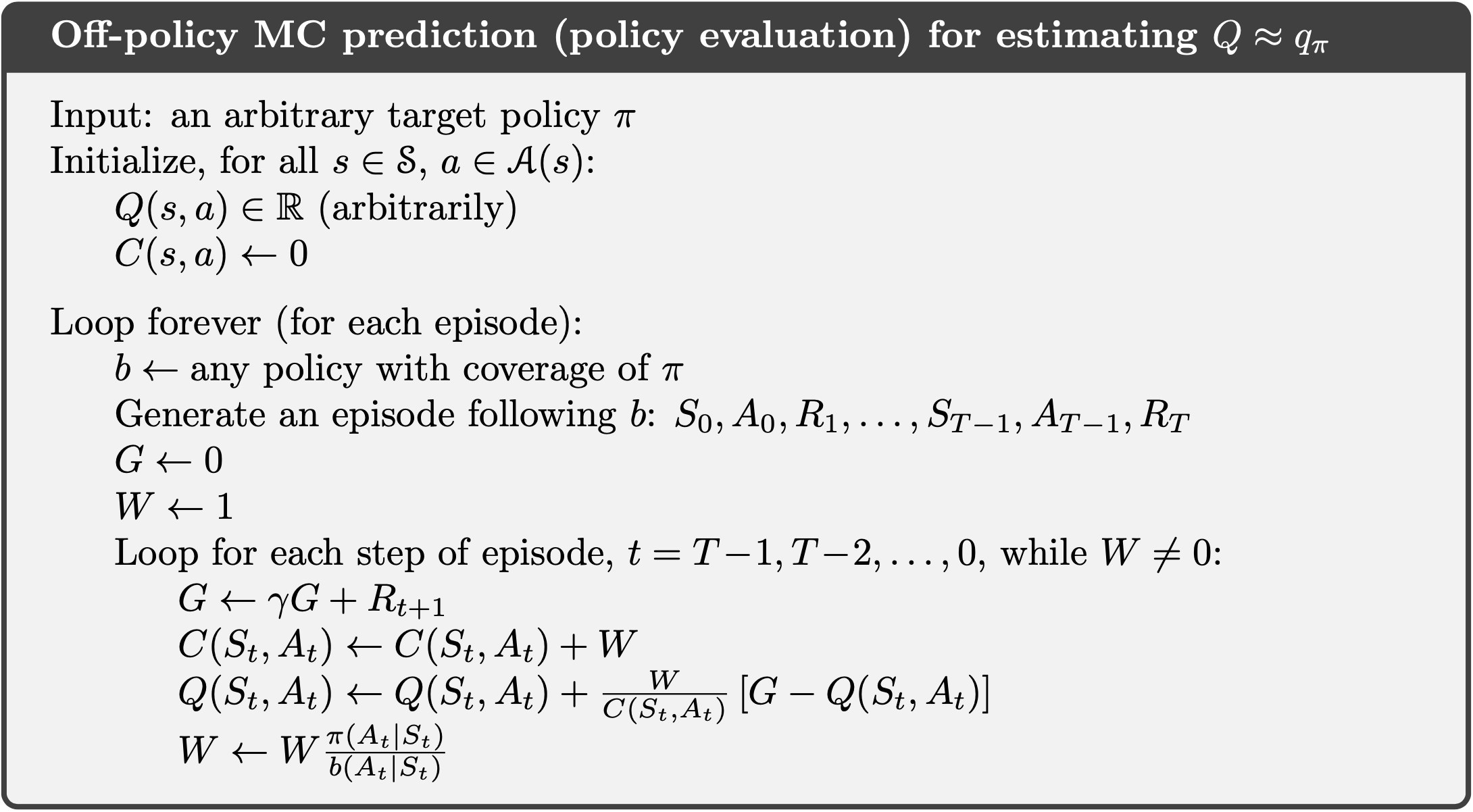
- Prediction problem: estimate $v_\pi$ or $q_\pi$ from episodes following a policy $b\neq \pi$ where $\pi$ is the target policy and $b$ is the behavior policy.
- The assumption of coverage: require that every action taken under $\pi$ is also taken under $b$.
\[\pi(a\mid s)>0 \rightarrow b(a\mid s)>0\]
- Importance sampling: a general technique for estimating expected values under one distribution given samples from another.
- Given a stating state $S_t$ and the subsequent state-action trajectory $A_t, S_{t+1}, A_{t+1},…, S_T$, the importance sampling ratio is
\[\p_{t:T-1}=\frac{\prod_{k=t}^{T-1}\pi(A_k\mid S_k)p(S_{k+1}\mid S_k,A_k)}{\prod_{k=t}^{T-1}b(A_k\mid S_k)p(S_{k+1}\mid S_k,A_k)}=\prod_{k=t}^{T-1}\frac{\pi(A_k\mid S_k)}{b(A_k\mid S_k)}\]
- The returns $G_t$ due to the behavior policy have the undesired expectation $E[G_t\mid S_t=s]=v_b(s)$.
- The ratio transforms the returns to have the desired expected value
\[E[\p_{t:T-1}G_t\mid S_t=s]=v_\pi(s)\]
- Ordinary importance sampling: scale the returns by the ratios and average the results
\[v_\pi(s)=\frac{\sum_{t\in \T(s)} \p_{t:T(t)-1} G_t}{\mid \T(s)\mid} \text{ where } \mathbb{T}(s) = \{t \mid S_t = s\}\]
- Weighted importance sampling:
\[v_\pi(s)=\frac{\sum_{t\in \T(s)}\p_{t:T(t)-1}G_t}{\sum_{t\in \T(s)}\p_{t:T(t)-1}}\]
- For first-visit methods, ordinary importance sampling is unbiased whereas weighted important sampling is biased. Variance of ordinary importance sampling is in general unbounded because the variance of the ratios can be unbounded. Weighted estimator usually has dramatically lower variance and is strongly preferred.
- Ordinary importance sampling can be more easily extended to the approximate methods using function approximation.
- For every-visit methods, ordinary and weighted importance sampling are both biased.
- In practice every-visit methods are often preferred because they remove the need to keep track of which states have been visited and because they are much easier to extend to approximations
- Weighted importance sampling for $q$
\[Q_(s,a)=\frac{\sum_{t\in \T(s,a)}\p_{t+1:T(t)-1}G_t}{\sum_{t\in \T(s,a)}\p_{t+1:T(t)-1}}\]
5.6 Incremental Implementation
- Incrementally average the returns
- Ordinary importance sampling: the returns are scaled by the importance sampling ratio, then simply averaged. We can use the incremental formulas for updating reward average, using the scaled returns in place of the rewards.
- Weighted importance sampling: Suppose we have returns $G_1,G_2,…,G_{n-1}$ and weights $W_1,W_2,…,W_{n-1}$ where $W_i=\p_{t_i:T(t_i)-1}$.
\[V_{n+1}=V_n+\frac{W_n}{C_n}[G_n-V_n]\]
\[C_{n+1}=C_n+W_{n+1} \text{ where } C_0=0\]
- The algorithm is nominally for the off-policy case, using weighted importance sampling, but applies as well to the on-policy case just by choosing the target and behavior policies as the same (in which case $\pi=b$, $W$ is always $1$).
- The approximation $Q$ converges to $q_\pi$ (for all encountered state-action pairs) while actions are selected according to a potentially different policy, $b$.
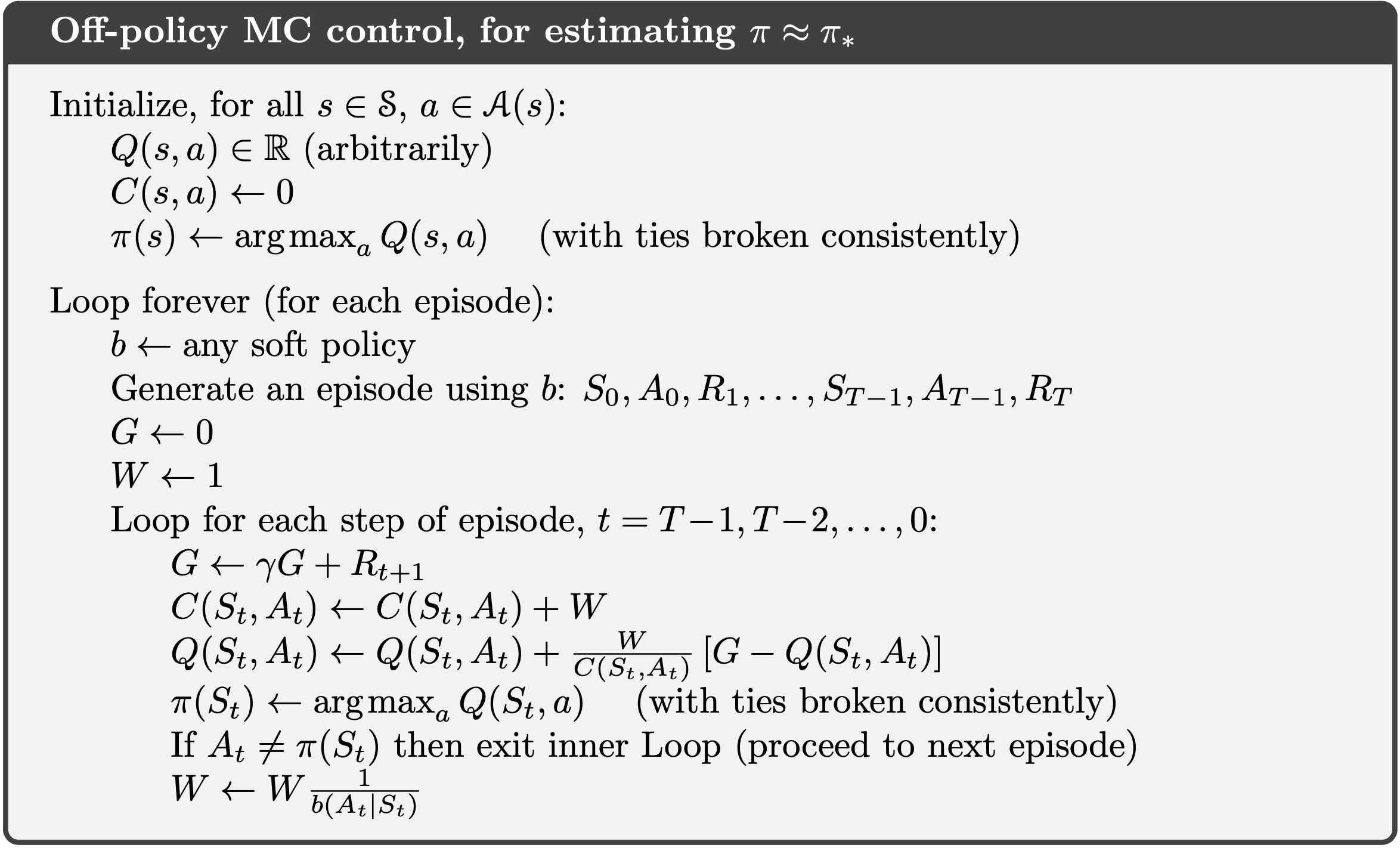
5.7 Off-policy Monte Carlo Control
- In off-policy methods, the behavior policy may in fact be unrelated to the target policy.
- An advantage of this is that the target policy may be deterministic, while the behavior policy can continue to sample all possible actions.
- Requires that the behavior policy has a nonzero probability of selecting all actions that might be selected by the target policy (coverage).
- To explore all possibility, we require that the behavior policy be soft (i.e. that it select all actions in all states with nonzero probability).
References
- Richard S. Sutton and Andrew G. Barto. Reinforcement Learning: An Introduction; 2nd Edition. 2017.